What if a photograph could be the starting point for exploring a heritage collection? Our reverse image search proof of concept began with finding related images in BALaT. It has grown into an experiment in letting researchers decide what “similar” should mean.
A collection can contain an overall view of an object, photographs of its details, and reproductions made under different conditions. Finding these connections through catalogue text depends on what has been described and how. Visual search offers another way in: start with an image and look for photographs that resemble it.
This post follows the development recorded in our experiment notes, from the first working tests on 28 June 2026 to the 343-image prototype shown here.
Starting from an existing approach
Our starting point was the image-search approach of PHAROS / artresearch.net, presented by Artem Kozlov at the 62nd CIDOC CRM SIG meeting in March 2026. His artresearch.net presentation (PDF) identifies SigLIP 2 and USearch as components of that system. We used this technical presentation as our architectural reference, then implemented and extended the visual-search approach for our own collection.
The underlying model is described in the research paper SigLIP 2: Multilingual Vision-Language Encoders with Improved Semantic Understanding, Localization, and Dense Features by Michael Tschannen and colleagues (2025). These are two distinct sources: PHAROS provided the heritage-search reference; the SigLIP 2 paper describes the model we use.
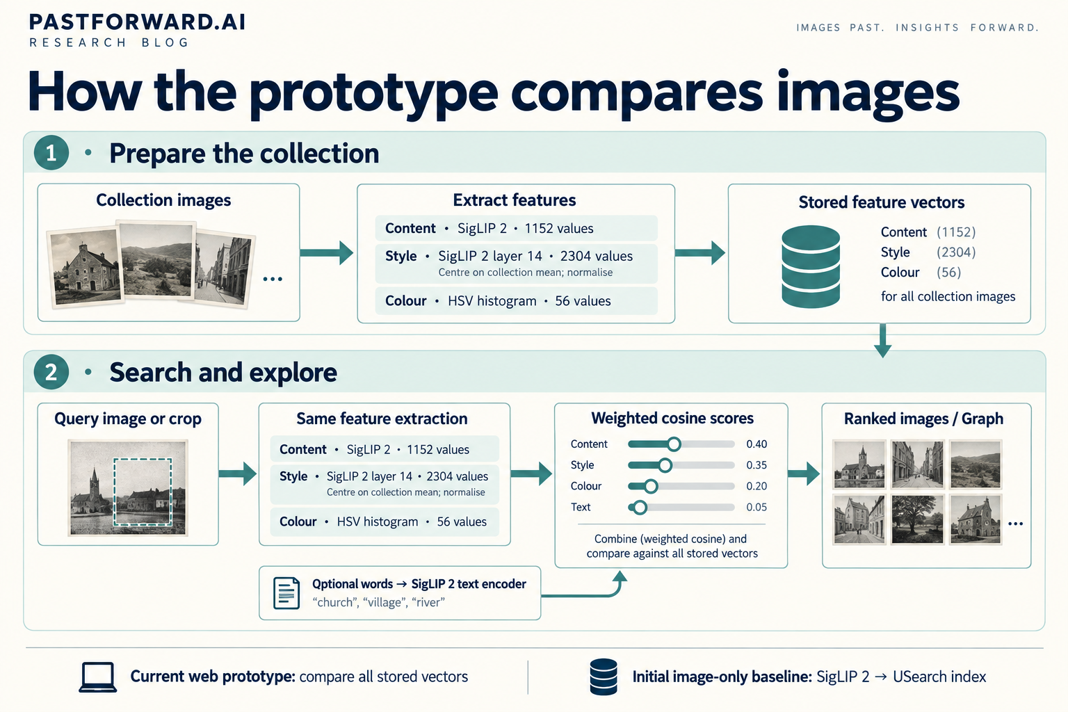
The principle is straightforward. A model turns each collection image into a numerical representation, called an embedding. It does the same for a query image, then searches for nearby representations in the index. The output is a ranked set of images for a person to inspect.
We chose the SigLIP 2 NaFlex model, which supports image and text representations and adapts to different image shapes and resolutions. Our prototype runs the model locally on a single workstation. Once the weights and collection images are downloaded, searches can run without sending images to an external AI service.
The model and components we actually use
The current prototype uses one pretrained model checkpoint: google/siglip2-so400m-patch16-naflex. Its image and text encoders serve different roles within the same model. We use the published weights without fine-tuning.
| Component | Role in the prototype | Representation |
|---|---|---|
| SigLIP 2 image encoder | Main content similarity, using the pooled image output | 1,152 values per image |
| SigLIP 2 text encoder | Text search and optional steering, compared against image content vectors | 1,152 values per prompt |
| SigLIP 2 intermediate features | Experimental style descriptor: mean and standard deviation of layer-14 features over valid image patches | 2,304 values per image |
| HSV colour histogram | Colour distribution, calculated directly from pixels; no additional AI model | 56 values per image |
| USearch | Approximate nearest-neighbour index for the initial image-only search; a search engine, not a model | Indexes the 1,152-value content vectors |
NaFlex adapts the image preprocessing to its aspect ratio, using 16 × 16 pixel patches. Our configuration allows up to 256 patches per image. The encoder pools the visual features into a fixed-length vector, which we L2-normalise: divide it by its length. For normalised vectors, a dot product gives cosine similarity, measuring alignment rather than vector magnitude.
We run the model through PyTorch and Hugging Face Transformers, using bfloat16 on the GPU and storing features as float32 arrays. The colour descriptor joins a 12 × 4 hue–saturation histogram with eight brightness bins: 48 + 8 = 56 values. The style descriptor joins 1,152 means and 1,152 standard deviations, excluding padded patches, then subtracts the collection mean and normalises the result.
DINOv2 remains a possible comparison model. PHAROS’s separate Qwen-based metadata search is outside this prototype; our text steering already uses SigLIP 2’s own text encoder.
A first test with 303 images
We began with 303 images from KIK-IRPA’s IIIF image service. One useful early test involved a detail photograph of a carved oak church cabinet. The index contained an 800-pixel version; we queried it with a 400-pixel version of the same photograph.
The matching photograph came first, with a similarity score of about 0.87. Other photographs of the cabinet followed, including a fuller view at about 0.69. This gave us an encouraging example of both resolution tolerance and a connection between a detail and the wider object.
The distinction matters: changing the resolution of an indexed photograph is a limited test. The neighbouring cabinet views were useful qualitative evidence, but this was still a small experiment, with results checked visually. It did not establish an accuracy rate for the collection.
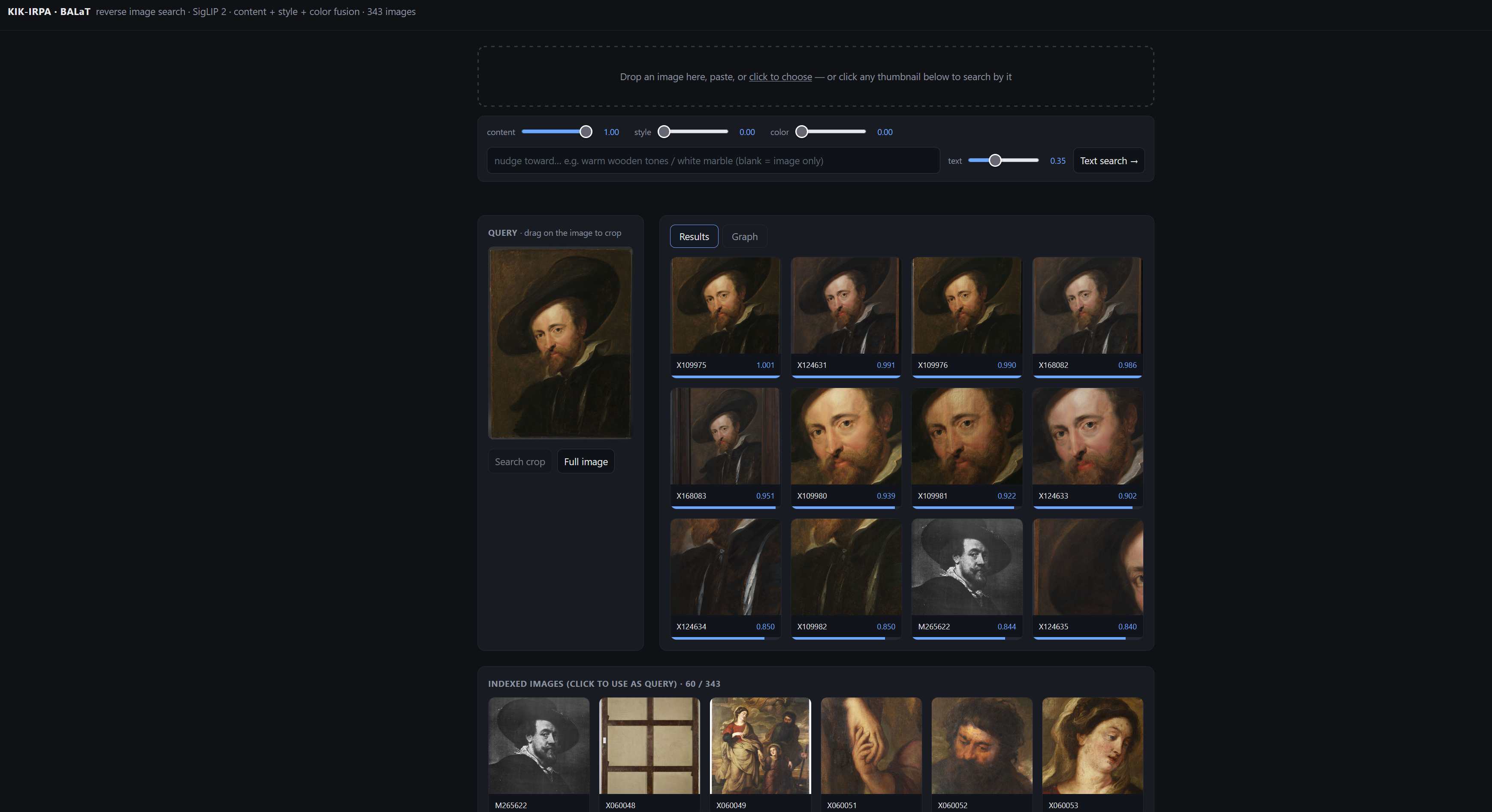
We then made the search easier to explore through a browser: upload or paste an image, or select an indexed thumbnail, and inspect the ranked results. The later test set grew to 343 images.
Giving the researcher a say in similarity
A single ranking quickly raises a question: similar in what way? A researcher might be interested in the subject, a colour palette, a surface texture or a particular detail. One embedding combines several of these signals, without giving the user separate controls.
We first added a text prompt to steer the search. A phrase such as “wooden carved cabinet” can retrieve images directly, or help reorder image-search results. This uses the text encoder of the same model. On our small test collection, text steering sometimes changed the order only subtly: a prompt cannot retrieve examples that the collection does not contain.
Next came separate content, style and colour sliders. Content uses the main image representation; colour compares colour distributions; the experimental style channel uses statistics from an intermediate model layer as a proxy for visual texture and appearance. Adjusting their weights produces different neighbours without retraining the model.
The style experiment needed a correction. Its initial representations shared such a strong common component that differences between images were hard to distinguish. Subtracting the dataset average before comparison made that channel more discriminating. It is still an experimental visual descriptor, not an art-historical classification of style.
Separate vectors, combined scores
We keep each feature channel separate throughout storage and comparison. The current features.npz file contains three aligned arrays: semantic with shape N × 1,152, style with shape N × 2,304, and color with shape N × 56. Row i refers to the same image in each array, identified by the accompanying paths list. The saved style_mean ensures that a new query is centred against exactly the same collection average.
These are separate vectors within one storage file, rather than one concatenated vector or three independent databases. Text prompts are encoded when needed and cached in memory; their vectors are compared with the stored content array.
For each candidate image, we calculate a content score, a style score and a colour score in their respective spaces. An optional fourth score compares the text prompt with that candidate’s content vector. We then take a weighted average of the active scores:
score = (w_content × s_content + w_style × s_style
+ w_colour × s_colour + w_text × s_text)
/ (w_content + w_style + w_colour + w_text)
Here, each s is a cosine similarity and each w is a slider weight. Channels with zero weight, missing query features, or an empty text prompt are omitted from both the numerator and denominator. If no channel is active, the implementation falls back to content similarity, or text similarity for a text-only query.
For example, suppose one image scores 0.80 for content and 0.40 for colour. With weights of 3 for content and 1 for colour, its combined score is (3 × 0.80 + 1 × 0.40) / 4 = 0.70. Reversing the weights gives 0.50. A second image with a closer palette can therefore move ahead when the researcher raises the colour weight.
This is often called late fusion: combine the scores after comparing the features. A fixed merged vector would bake a particular balance into the representation. Keeping the channels separate makes it easy to change that balance, disable a channel, or inspect its contribution without extracting the collection features again. It also accommodates the different vector lengths without treating a larger descriptor as automatically more important.
A carefully normalised and weighted concatenation could reproduce this weighted-cosine calculation. Our choice is about explicit control and simpler experimentation: the saved descriptors remain independent, and the slider settings belong to the query.
In the current web app, NumPy matrix–vector products compute each channel’s scores across every stored image, and the combined scores determine the ranking. At 343 images this is practical. Larger collections will need measured strategies for candidate retrieval and reranking. The channels also have different score distributions: normalisation makes cosine comparison possible, but does not calibrate the channels to equal influence. In particular, text–image scores can be lower than image–image scores, so the weights need evaluation.
Searching from a detail
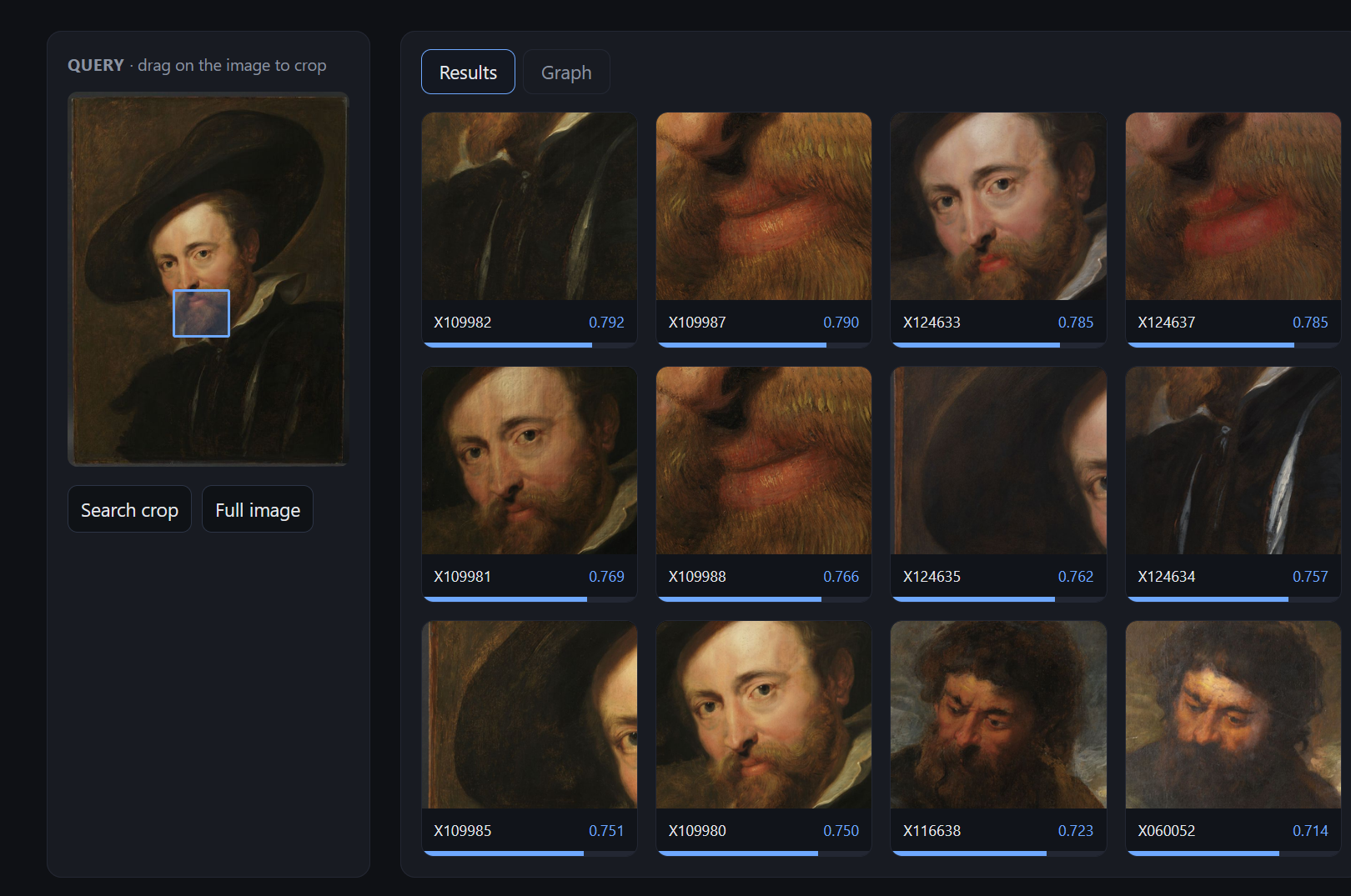
Another useful control was simpler: let the researcher choose the part of the photograph that matters. We added a rectangle selection so a query can use a crop, with the same content, style, colour and text controls available afterwards.
In the example below, the selection focuses on the mouth and beard within a portrait. The ranking brings up several close details alongside broader portrait views and other bearded faces. It shows how a change in the query region changes the search question—and why the returned images still need interpretation.
From a results grid to a network
A ranked grid answers “what is close to this image?” We also wanted to explore what lies beyond those first matches. The graph view starts from a query, finds neighbouring images, then expands through their neighbours. Clicking a node makes it the new starting point.
The first version exposed a problem familiar to photographic archives: several very similar photographs kept leading back to one another. The graph formed a small ring instead of opening onto the wider collection.
We changed expansion to exclude images already shown, so each level reaches new photographs. We then added cross-links between sufficiently similar images to keep clusters visible. The prototype caps the network at 48 image nodes and lets the user adjust its depth and number of neighbours, zoom, pan and explore it in an expanded view.
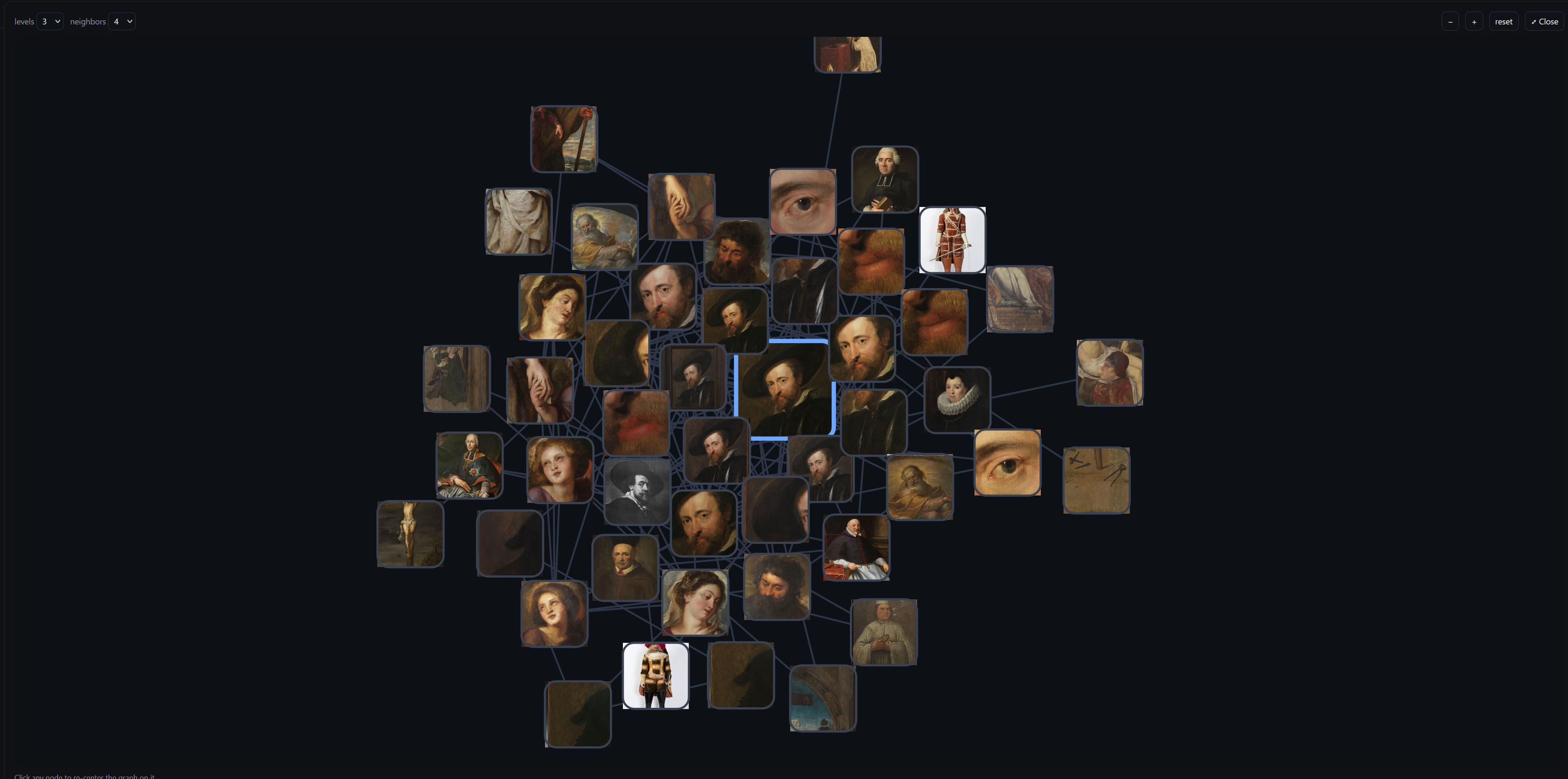
The links represent visual similarity under the search settings. They offer leads for investigation; they do not establish authorship, provenance or a historical relationship between the depicted works.
What hardware would another institution need?
Reusing this method involves two workloads: preparing collection features, then running searches against them. They can run on different machines. A GPU can accelerate the initial preparation; the saved vectors can then be moved to a CPU server. Our code selects CUDA when available and otherwise runs the model on CPU.
Our experiments used an RTX 4090 with 24 GB of GPU memory, and CPU measurements used a 28-core machine. We have not established a minimum hardware specification through tests on smaller machines. The configurations below are practical starting estimates for evaluation, with small batches and few simultaneous users.
| Workload | Starting configuration to evaluate | What determines capacity? |
|---|---|---|
| Reproduce the small prototype | A modern multicore CPU, 16 GB RAM and an SSD; no dedicated GPU required by the code | Model loading and feature extraction dominate. Start with batch size 1 and allow more time on CPU. |
| Prepare a larger collection | 8–16 CPU cores, 32 GB RAM, SSD storage and a compatible NVIDIA GPU with 8–12 GB VRAM as a small-batch target | Actual GPU memory use depends on batch size and intermediate features. Our validated GPU had 24 GB; smaller cards still need testing. |
| Serve a modest collection internally | 8–16 CPU cores, 16–32 GB RAM and an SSD; GPU optional | Allow memory for the model, feature arrays and request processing. Size against the collection and measure concurrent searches. |
| Plan for roughly one million images | Evaluate 32–64 GB RAM for a redesigned service retaining all three float32 feature channels | This is a capacity estimate, not a tested deployment. Efficient candidate retrieval, graph expansion and memory use need further work. |
The preparation step downloads or reads image derivatives, decodes them, extracts features and saves the vectors. Our model download is roughly 4.3 GB; allow additional SSD space for the Python environment, temporary files and images. For example, 980,000 derivatives averaging 120 KB would occupy about 118 GB in decimal units. Image acquisition can take longer than inference when requests must respect an image server’s rate limits.
The current scripts read a local image folder. Streaming images from IIIF and serving remote thumbnails could reduce permanent image storage, but would require adapting this workflow. Large-scale feature preparation also needs incremental writes: the prototype accumulates arrays in memory, so peak RAM can exceed the final feature-file size substantially.
How much space do the vectors need?
A separate vector-database server is not required for this prototype. The original baseline uses an embedded USearch index and an image lookup file. The current multi-channel web app loads its separate NumPy feature arrays from features.npz.
The raw storage calculation is straightforward: number of images × values per image × bytes per value. With float32 storage, content alone uses 1,152 × 4 = 4,608 bytes per image. Keeping content, style and colour separately uses (1,152 + 2,304 + 56) × 4 = 14,048 bytes per image.
| Images | Content only, float32 | All three channels, float32 |
|---|---|---|
| 343 | 1.58 MB | 4.82 MB |
| 100,000 | 461 MB | 1.40 GB |
| 980,000 | 4.52 GB | 13.77 GB |
These calculated figures use decimal MB and GB and exclude index structures, image identifiers, the style mean, model weights, images, backups and working memory. USearch supports reduced-precision storage and memory-mapped indexes, but those options do not automatically reduce the current web app’s float32 arrays. Storage savings and retrieval quality would need to be assessed together.
Preparing once, serving elsewhere
A useful deployment pattern is to prepare the features on a GPU workstation and transfer them to an internal CPU server. For the current web app, the transfer must include features.npz, its saved style mean and image mapping, the model and processor files, and accessible image files with matching paths. The baseline’s USearch index alone is insufficient for the multi-channel interface.
Choosing an already indexed image reuses its stored features. A new upload, crop or text prompt needs model inference. Our notes record roughly 426 ms for CPU image embedding on the 28-core test machine using 14 threads. This is a measured component time, not a guarantee for a smaller CPU or for the complete multi-channel search and graph response.
Turning the research interface into a shared service also requires an application server, institutional access controls, backups and monitoring. The prototype’s Python HTTP server is a development interface. At collection scale, candidate retrieval and reranking must replace repeated full-array scans where needed; enough RAM to hold the vectors does not by itself ensure responsive searches.
To make a future code release reproducible, the method should travel with the code: the exact model revision, locked dependencies, preprocessing settings, feature dimensions, style-centering data, score formula, sample commands and evaluation queries. Hardware, batch size, numerical precision and measured timings belong in that record too. A receiving institution should rebuild the software environment for its own CPU or GPU rather than copy a workstation’s virtual environment.
Where we are now
We have a working local prototype that combines image search, text search and steering, adjustable similarity channels, detail crops and a navigable graph. The screenshots capture that prototype with 343 indexed images. They illustrate its behaviour, rather than a benchmark of retrieval quality. The displayed similarity scores are ranking signals, not probabilities that two images depict the same object.
The next step is a larger and more varied corpus, together with expert-judged queries that distinguish different tasks: finding another photograph of the same object, connecting a detail to a whole, or exploring a broader visual resemblance. We need to measure how reliably useful matches appear near the top and examine the failures.
Our scaling notes also separate the cost of preparing a collection from the cost of searching it. The initial image index uses USearch; the current browser prototype blends its multiple similarity channels by comparing all stored feature vectors. Moving that richer search to collection scale will require further indexing work and measurement. The notes explore a collection of roughly 980,000 images as a planning scenario, not a completed deployment.
Automatic object masking and a comparison with a second visual model remain possible experiments. For now, the progress is concrete: a researcher can start from a photograph, narrow the question to a detail, change the basis of comparison and follow the results into a wider group of images.
← All posts